Code
lapply(
  X = setdiff(
    c("whitebox", "terra", "sf", "ggplot2", "tidyterra", "scico"),
    installed.packages()[, "Package"]),
FUN = install.packages)list()Spatial Data Science
Geocomputation with R
In this session we use the WhiteboxTools (WBT) a modern and advanced geospatial package, tools collection, which contains ~450 functions. The WBT has an interface to both R and Python.
The tool can be downloaded from http://whiteboxgeo.com/. We have to install through the packge. First the necessary packages need to be installed, the installation require compilation and take some time. ## Raster and vector data
Raster data are represented by a matrix of pixels (cells) with values. Raster is used for data which display continuous information across an area which cannot be easily divided into vector features. For the purpose of watershed delineation the raster input of Digital Elevation Model is used.
The process of delineation is the first step in basin description. One simply has to delineate the domain
The step-by-step process involves:
Let’s start with whitebox package that contains an API to the WhiteboxTools executable binary.
We need to reference path to the executable
Except for the whitebox package, some other packages for general work with spatial data are necessary. The packages terra and sf are needed for working with the raster and vector data. They also provide access to PROJ, GEOS and GDAL which are open source libraries that handle projections, format standards and provide geoscientific calculations. And the package tmap makes plotting both raster and vector layers very easy.
We will install the whitebox tools through the whitebox package. Other than this package we will need the sf and terra in order to deal with the vector and raster data formats and ggplot2 for general visualisation and map-making.
We have to install the sought packages prior the first usage. None of them is actually contained in the default R installation.
lapply(
X = setdiff(
c("whitebox", "terra", "sf", "ggplot2", "tidyterra", "scico"),
installed.packages()[, "Package"]),
FUN = install.packages)list()After the successful installation, the library function load the namespace of the packages and allows their exported functions to be used directly.
library(whitebox)
library(terra)
## terra 1.8.60
library(sf)
## Linking to GEOS 3.13.0, GDAL 3.8.5, PROJ 9.5.1; sf_use_s2() is TRUE
library(ggplot2)
library(tidyterra)
##
## Attaching package: 'tidyterra'
## The following object is masked from 'package:stats':
##
## filter
library(scico)terra package for raster use.
sf package for vector use.
ggplot2 plotting functions for layers.
tidyterra for the terra objects and ggplot2 compatibility.
The paths on your OS may vary, you may need to change the direction of the installation.
wd_path <- "~/Desktop/GIS"
wbt_init(exe_path = paste(wd_path, "WBT/whitebox_tools", sep = "/"))
check_whitebox_binary()
## [1] TRUETRUE if found.
dem <- rast(whitebox::sample_dem_data())
writeRaster(dem, paste(wd_path, "dem.tif", sep = "/"), overwrite = TRUE)
ggplot() +
geom_spatraster(data = dem) +
scale_fill_scico(palette = "turku")rast() function to load the data
tmap workflow
The digital elevation model has to be adjusted for the watershed delineation algorithm to be able to run successfully.
It’s good to specify a path to working directory. It has to be somewhere where you as a user have access to write files. Be sure the folder exists.
wbt_fill_depressions_wang_and_liu(dem = paste(wd_path,
"dem.tif",
sep = "/"),
output = paste(wd_path,
"filled_depresions.tif",
sep = "/"))
wbt_d8_pointer(dem = paste(wd_path,
"filled_depresions.tif",
sep = "/"),
output = paste(wd_path,
"d8pointer.tif",
sep = "/"))
wbt_d8_flow_accumulation(input = paste(wd_path,
"filled_depresions.tif",
sep = "/"),
output = paste(wd_path,
"flow_accu.tif",
sep = "/"),
out_type = "cells")
wbt_extract_streams(flow_accum = paste(wd_path,
"flow_accu.tif",
sep = "/"),
output = paste(wd_path,
"streams.tif",
sep = "/"),
threshold = 200)
We have the raster prepared for the delineation, now we need to provide a point layer with the gauge, to which the watershed should be delineated. The point has to be placed at the stream network. We will create the layer from scratch.
gauge <- st_sfc(st_point(x = c(671035, 4885783),
                               dim = "XY"),
                      crs = st_crs(26918))
st_write(gauge, dsn = paste(wd_path, "gauge",
                            sep = "/"),
         driver = "ESRI Shapefile",
         append = FALSE)
Deleting layer `gauge' using driver `ESRI Shapefile'
Writing layer `gauge' to data source
`/Users/petrmbpro/Desktop/GIS/gauge' using driver `ESRI Shapefile'
Writing 1 features with 0 fields and geometry type Point.ggplot() +
geom_spatraster(data = dem) +
scico::scale_fill_scico(palette = "turku") +
geom_sf(data = gauge, color = "orangered")If the point is not located directly in the stream, it could cause troubles. The Jenson snap pour makes sure to move the point to the nearest stream pixel.
wbt_jenson_snap_pour_points(pour_pts = paste(wd_path,
                                             "gauge/gauge.shp",
                                             sep = "/"),
                            streams = paste(wd_path,
                                            "streams.tif",
                                            sep = "/"),
                            output = paste(wd_path,
                                           "gauge_snapped.shp",
                                           sep = "/"),
                            snap_dist = 1000)
Now everything is set to delineate the watershed with using the gauge and D8 pointer.
wbt_watershed(d8_pntr = paste(wd_path, "d8pointer.tif", sep = "/"),
              pour_pts = paste(wd_path, "gauge_snapped.shp", sep = "/"),
              output = paste(wd_path, "watershed.tif", sep = "/"))
The watershed is usually used in vector format, but now it is in raster. Let’s finish with the conversion.
wtshd <- rast(paste(wd_path, "watershed.tif", sep = "/"))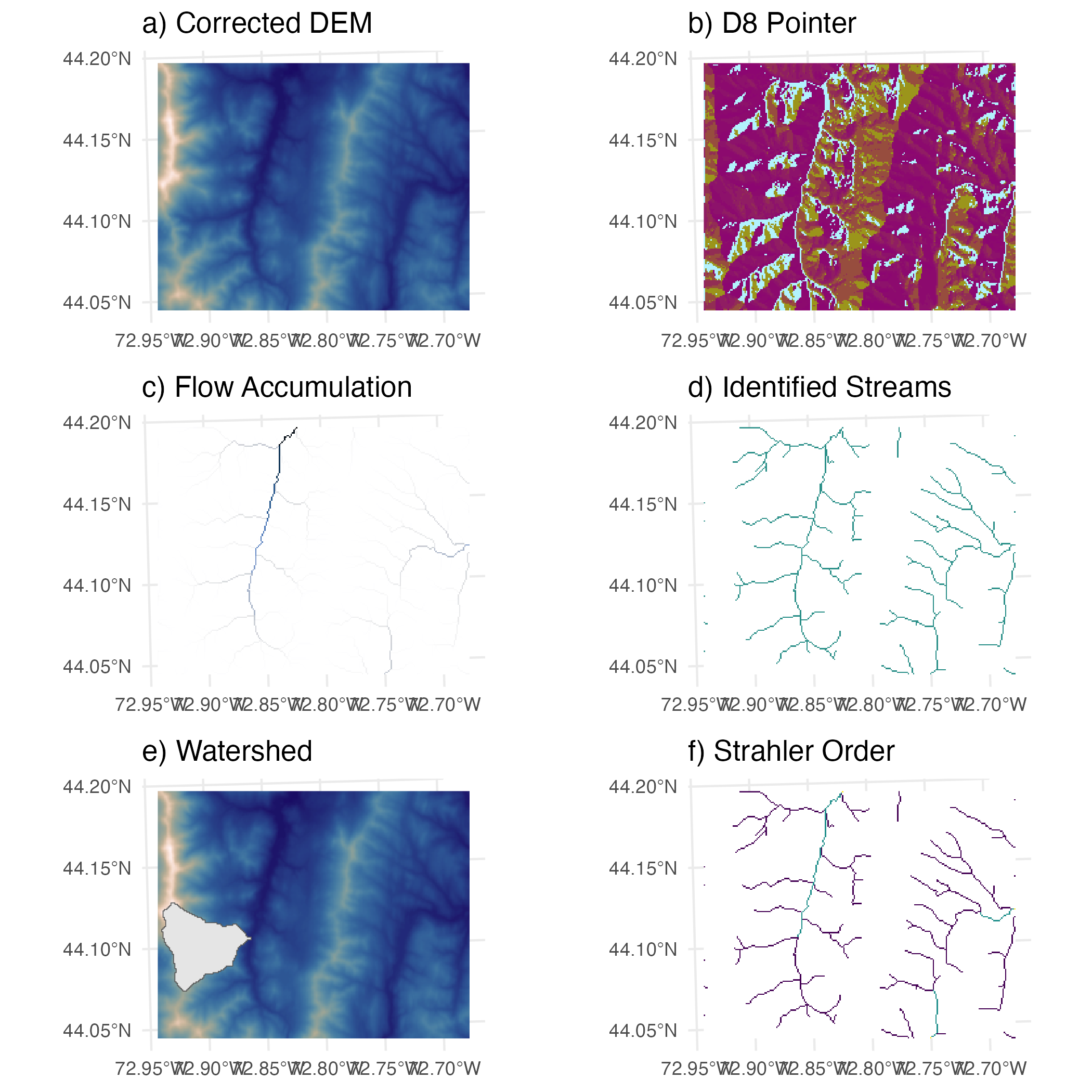
watershed <- terra::as.polygons(wtshd)Under the term river morphology we understand the description of the shape of river channels. Hydrologists use indices such as stream length or Strahler order.
wbt_strahler_stream_order(d8_pntr = paste(wd_path, "d8pointer.tif", sep = "/"),
                          streams = paste(wd_path, "streams.tif", sep = "/"),
output = paste(wd_path, "strahler.tif", sep = "/"))results <- list.files(wd_path, pattern = "tif$", full.names = TRUE)
r <- lapply(results, rast)
r1 <- rast(results[2])
r2 <- rast(results[1])
r3 <- rast(results[4])
r4 <- rast(results[6])
r5 <- watershed
r6 <- rast(results[5])
p1 <- ggplot() +
ggtitle(label = "a) Corrected DEM") +
geom_spatraster(data = r1, show.legend = FALSE) +
scale_fill_scico(palette = "lapaz") +
theme_minimal()
p2 <- ggplot() +
ggtitle(label = "b) D8 Pointer") +
geom_spatraster(data = r2, show.legend = FALSE) +
scale_fill_scico(palette = "hawai") +
theme_minimal()
p3 <- ggplot() +
ggtitle(label = "c) Flow Accumulation") +
geom_spatraster(data = r3, show.legend = FALSE) +
scale_fill_scico(palette = "oslo", direction = -1) +
theme_minimal()
p4 <- ggplot() +
ggtitle(label = "d) Identified Streams") +
geom_spatraster(data = r4, show.legend = FALSE) +
scale_fill_viridis_c(na.value = "white") +
theme_minimal()
p5 <- ggplot() +
ggtitle(label = "e) Watershed") +
geom_spatraster(data = r1, show.legend = FALSE) +
scale_fill_scico(palette = "lapaz") +
geom_spatvector(data = r5, show.legend = FALSE) +
theme_minimal()
p6 <- ggplot() +
ggtitle(label = "f) Strahler Order") +
geom_spatraster(data = r6, show.legend = FALSE) +
scale_fill_viridis_b(na.value = "white") +
theme_minimal()
cowplot::plot_grid(p1, NULL, p2,
p3, NULL, p4,
p5, NULL, p6,
nrow = 3, align = "hv", rel_widths = c(1,0,1), greedy = TRUE)