3 GIS in Hydrology

Spatial Data Science
Geocomputation with R

3.1 WhiteboxTools

In this session we use the WhiteboxTools (WBT) a modern and advanced geospatial package, tools collection, which contains ~450 functions. The WBT has an interface to r and python.

The tool can be downloaded from http://whiteboxgeo.com/.

3.2 Raster and vector data

Raster data are represented by a matrix of pixels (cells) with values. Raster is used for data which display continuous information across an area which cannot be easily divided into vector features. For the purpose of watershed delineation the raster input of Digital Elevation Model is used.

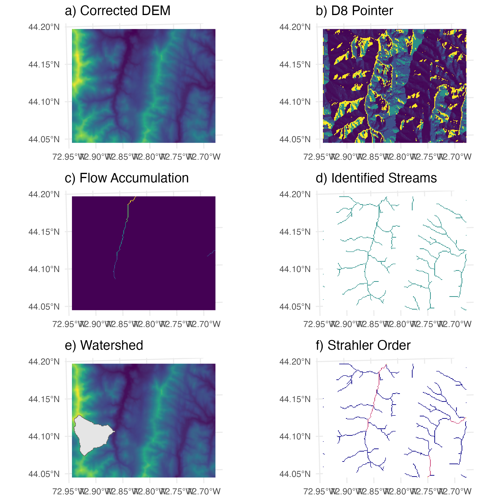
3.3 Watershed delineation

The process of delineation is the first step in basin description. One simply has to delineate the domain

The step-by-step process involves:

Acquiring digital elevation model of area
Pit and sink removal
Flow accumulation calculation
Flow direction calculation
Outlet identification
Delineation towards specified outlet

Let’s start with whitebox package that contains an API to the WhiteboxTools executable binary.
We need to reference path to the executable

Except for the whitebox package, some other packages for general work with spatial data are necessary. The packages terra and sf are needed for working with the raster and vector data. They also provide access to PROJ, GEOS and GDAL which are open source libraries that handle projections, format standards and provide geoscientific calculations. And the package tmap makes plotting both raster and vector layers very easy.

3.4 Watershed delineation workflow

Code

library(whitebox)
library(terra)
## terra 1.7.55
library(sf)
## Linking to GEOS 3.11.0, GDAL 3.5.3, PROJ 9.1.0; sf_use_s2() is TRUE
library(tmap)
## Breaking News: tmap 3.x is retiring. Please test v4, e.g. with
## remotes::install_github('r-tmap/tmap')
whitebox::wbt_init(exe_path = "~/Downloads/WBT/whitebox_tools")
whitebox::check_whitebox_binary()
## [1] TRUE

1: Load the Whitebox API package
2: Load the terra package for raster use
3: Load the sf package for vector use
4: Load the tmap plotting functions for layers
5: Whitebox needs the information where the data executable is stored
6: Binary check of functionality

3.4.0.1 Sample data

Code

dem <- rast(whitebox::sample_dem_data())
tm_layout() +
  tm_shape(dem) +
  tm_raster(palette = "-Greys", n = 50, legend.show = FALSE)

1: Use the rast() function to load the data
2: Plot via the tmap workflow

3.4.0.2 DEM workflow

The digital elevation model has to be adjusted for the watershed delineation algorithm to be able to run successfully.

We need to specifiy a path to working directory. It has to be somewhere where you as a user have access to write files. Be sure the folder exists.

Code

wd_path <- "~/Desktop/GIS"

Code


wbt_fill_depressions_wang_and_liu(dem = paste(wd_path,
                                              "dem.tif",
                                              sep = "/"),
                                  output = paste(wd_path,
                                                 "filled_depresions.tif",
                                                 sep = "/"))

wbt_d8_pointer(dem = paste(wd_path,
                           "filled_depresions.tif",
                           sep = "/"),
               output = paste(wd_path,
                              "d8pointer.tif",
                              sep = "/"))

wbt_d8_flow_accumulation(input = paste(wd_path,
                                       "filled_depresions.tif",
                                       sep = "/"),
                         output = paste(wd_path,
                                        "flow_accu.tif",
                                        sep = "/"),
                         out_type = "cells")

wbt_extract_streams(flow_accum = paste(wd_path,
                                       "flow_accu.tif",
                                       sep = "/"),
                    output = paste(wd_path,
                                   "streams.tif",
                                   sep = "/"),
                    threshold = 200)

1: This algorithm involves removing flat areas and filling depressions, thus producing hydrologically corrected DEM
2: Pointer is

3.4.1 Gauge

We have the raster prepared for the delineation, now we need to provide a point layer with the gauge, to which the watershed should be delineated. The point has to be placed at the stream network. We will create the layer from scratch.

Code

gauge <- st_sfc(st_point(x = c(671035, 4885783), 
                               dim = "XY"), 
                      crs = st_crs(26918))
st_write(obj = gauge, 
         dsn = paste(wd_path, "gauge", sep = "/"), 
         driver = "ESRI Shapefile", 
         delete_dsn = TRUE)

Deleting source `/Users/petrmbpro/Desktop/GIS/gauge' using driver `ESRI Shapefile'
Writing layer `gauge' to data source 
  `/Users/petrmbpro/Desktop/GIS/gauge' using driver `ESRI Shapefile'
Writing 1 features with 0 fields and geometry type Point.

Code

tm_layout() +
  tm_shape(dem) +
  tm_raster(palette = "-Greys", n = 50, legend.show = FALSE) +
  tm_shape(gauge) +
  tm_dots(col = "red", size = 1)

If the point is not located directly in the stream, it could cause troubles. The Jenson snap pour makes sure to move the point to the nearest stream pixel.

Code

wbt_jenson_snap_pour_points(pour_pts = paste(wd_path, 
                                             "gauge/gauge.shp", 
                                             sep = "/"), 
                            streams = paste(wd_path, 
                                            "streams.tif", 
                                            sep = "/"), 
                            output = paste(wd_path, 
                                           "gauge_snapped.shp", 
                                           sep = "/"), 
                            snap_dist = 1000)

Now everything is set to delineate the watershed with using the gauge and D8 pointer.

Code

wbt_watershed(d8_pntr = paste(wd_path, "d8pointer.tif", sep = "/"),
              pour_pts = paste(wd_path, "gauge_snapped.shp", sep = "/"), 
              output = paste(wd_path, "watershed.tif", sep = "/"))

The watershed is usually used in vector format, but now it is in raster. Let’s finish with the conversion.

Code

wtshd <- rast(paste(wd_path, "watershed.tif", sep = "/"))
watershed <- terra::as.polygons(wtshd)

3.5 River morphology

Under the term river morphology we understand the description of the shape of river channels. Hydrologists use indices such as stream length or Strahler order.

Code

wbt_strahler_stream_order(d8_pntr = paste(wd_path, "d8pointer.tif", sep = "/"), 
                          streams = paste(wd_path, "streams.tif", sep = "/"), 
                          output = paste(wd_path, "strahler.tif", sep = "/"))

3.6 Results